[논문 구현] PyTorch로 DenseNet(2017) 구현하고 학습하기

 이번 포스팅에서는 DenseNet을 파이토치로 구현하고 학습까지 해보겠습니다! 작업 환경은 Google Colab에서 진행했습니다.

 

 논문 리뷰는 아래 포스팅에서 확인하실 수 있습니다.

[논문 읽기] DenseNet(2017) 리뷰, Densely Connected Convolutional Networks

 

 전체 코드는 여기에서 확인하실 수 있습니다.

 

 모델을 구현하기 전에, colab mount와 라이브러리 import를 하겠습니다.

from google.colab import drive
drive.mount('densenet')

 

# import package

# model
import torch
import torch.nn as nn
import torch.nn.functional as F
from torchsummary import summary
from torch import optim

# dataset and transformation
from torchvision import datasets
import torchvision.transforms as transforms
from torch.utils.data import DataLoader
import os

# display images
from torchvision import utils
import matplotlib.pyplot as plt
%matplotlib inline

# utils
import numpy as np
from torchsummary import summary
import time
import copy

 

1. 데이터셋 불러오기

 데이터셋은 torchvision 패키지에서 제공하는 STL10 dataset을 이용하겠습니다. STL10 dataset은 10개의 label을 갖으며 train dataset 5000개, test dataset 8000개로 구성됩니다.

 

 데이터셋을 불러옵니다.

# specify path to data
path2data = '/content/densenet/MyDrive/data'

# if not exists the path, make the directory
if not os.path.exists(path2data):
    os.mkdir(path2data)

# load dataset
train_ds = datasets.STL10(path2data, split='train', download=True, transform=transforms.ToTensor())
val_ds = datasets.STL10(path2data, split='test', download=True, transform=transforms.ToTensor())

print(len(train_ds))
print(len(val_ds))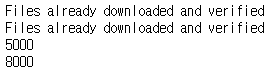

 

 transformation 객체를 정의하고 데이터셋에 적용하겠습니다. Resize(64)를 사용했는데, 더 큰 값을 사용해도 됩니다. 임의로 선택한 값입니다. 참고로 CIFAR dataset은 32x32, ImageNet dataset은 224x224의 크기를 갖습니다. 입력 이미지 크기가 작으면 모델의 파라미터 수가 감소합니다. 입력 이미지 크기가 크면 파라미터 수가 증가하는 대신에 더 높은 정확도를 얻을 수 있습니다.

# define transformation
transformation = transforms.Compose([
                    transforms.ToTensor(),
                    transforms.Resize(64)
])

# apply transformation to dataset
train_ds.transform = transformation
val_ds.transform = transformation

# make dataloade
train_dl = DataLoader(train_ds, batch_size=32, shuffle=True)
val_dl = DataLoader(val_ds, batch_size=32, shuffle=True)

 

 샘플 이미지를 확인합니다.

# check sample images
def show(img, y=None):
    npimg = img.numpy()
    npimg_tr = np.transpose(npimg, (1, 2, 0))
    plt.imshow(npimg_tr)

    if y is not None:
        plt.title('labels:' + str(y))

np.random.seed(7)
torch.manual_seed(0)

grid_size=4
rnd_ind = np.random.randint(0, len(train_ds), grid_size)

x_grid = [train_ds[i][0] for i in rnd_ind]
y_grid = [val_ds[i][1] for i in rnd_ind]

x_grid = utils.make_grid(x_grid, nrow=grid_size, padding=2)
plt.figure(figsize=(10,10))
show(x_grid, y_grid)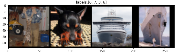

 

2. 모델 구축하기

 코드는 https://github.com/weiaicunzai/pytorch-cifar100/blob/master/models/densenet.py 를 참고했습니다.

 

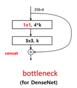
 우선 DenseNet에서 사용하는 BottleNeck을 정의합니다. 특이한 점은 residual과 shortcut을 add가 아닌 concat으로 연결합니다. 이 방법이 채널 수를 확장하기에 효율적인 방법입니다.

 

# DenseNet BottleNeck
class BottleNeck(nn.Module):
    def __init__(self, in_channels, growth_rate):
        super().__init__()
        inner_channels = 4 * growth_rate

        self.residual = nn.Sequential(
            nn.BatchNorm2d(in_channels),
            nn.ReLU(),
            nn.Conv2d(in_channels, inner_channels, 1, stride=1, padding=0, bias=False),
            nn.BatchNorm2d(inner_channels),
            nn.ReLU(),
            nn.Conv2d(inner_channels, growth_rate, 3, stride=1, padding=1, bias=False)
        )

        self.shortcut = nn.Sequential()

    def forward(self, x):
        return torch.cat([self.shortcut(x), self.residual(x)], 1)

 

 다음에는 Transition block을 정의합니다 Transition block은 Dense block 사이에 위치하며, 피쳐맵 크기와 채널 수를 절반으로 감소시킵니다.

# Transition Block: reduce feature map size and number of channels
class Transition(nn.Module):
    def __init__(self, in_channels, out_channels):
        super().__init__()

        self.down_sample = nn.Sequential(
            nn.BatchNorm2d(in_channels),
            nn.ReLU(),
            nn.Conv2d(in_channels, out_channels, 1, stride=1, padding=0, bias=False),
            nn.AvgPool2d(2, stride=2)
        )

    def forward(self, x):
        return self.down_sample(x)

 

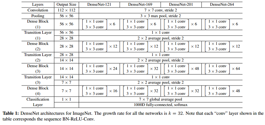
 이제 전체 구조를 정의합니다. 신경써야 할 것은 중간중간 inner channel이 계속해서 바뀌는 것입니다. 이전 레이어의 피쳐맵이 다음 모든 레이어에 합쳐지기 때문입니다.

 

 

# DenseNet
class DenseNet(nn.Module):
    def __init__(self, nblocks, growth_rate=12, reduction=0.5, num_classes=10, init_weights=True):
        super().__init__()

        self.growth_rate = growth_rate
        inner_channels = 2 * growth_rate # output channels of conv1 before entering Dense Block

        self.conv1 = nn.Sequential(
            nn.Conv2d(3, inner_channels, 7, stride=2, padding=3),
            nn.MaxPool2d(3, 2, padding=1)
        )

        self.features = nn.Sequential()

        for i in range(len(nblocks)-1):
            self.features.add_module('dense_block_{}'.format(i), self._make_dense_block(nblocks[i], inner_channels))
            inner_channels += growth_rate * nblocks[i]
            out_channels = int(reduction * inner_channels)
            self.features.add_module('transition_layer_{}'.format(i), Transition(inner_channels, out_channels))
            inner_channels = out_channels 
        
        self.features.add_module('dense_block_{}'.format(len(nblocks)-1), self._make_dense_block(nblocks[len(nblocks)-1], inner_channels))
        inner_channels += growth_rate * nblocks[len(nblocks)-1]
        self.features.add_module('bn', nn.BatchNorm2d(inner_channels))
        self.features.add_module('relu', nn.ReLU())

        self.avg_pool = nn.AdaptiveAvgPool2d((1,1))
        self.linear = nn.Linear(inner_channels, num_classes)

        # weight initialization
        if init_weights:
            self._initialize_weights()
    
    def forward(self, x):
        x = self.conv1(x)
        x = self.features(x)
        x = self.avg_pool(x)
        x = x.view(x.size(0), -1)
        x = self.linear(x)
        return x

    def _make_dense_block(self, nblock, inner_channels):
        dense_block = nn.Sequential()
        for i in range(nblock):
            dense_block.add_module('bottle_neck_layer_{}'.format(i), BottleNeck(inner_channels, self.growth_rate))
            inner_channels += self.growth_rate
        return dense_block

    def _initialize_weights(self):
        for m in self.modules():
            if isinstance(m, nn.Conv2d):
                nn.init.kaiming_normal_(m.weight, mode='fan_out', nonlinearity='relu')
                if m.bias is not None:
                    nn.init.constant_(m.bias, 0)
            elif isinstance(m, nn.BatchNorm2d):
                nn.init.constant_(m.weight, 1)
                nn.init.constant_(m.bias, 0)
            elif isinstance(m, nn.Linear):
                nn.init.normal_(m.weight, 0, 0.01)
                nn.init.constant_(m.bias, 0)

def DenseNet_121():
    return DenseNet([6, 12, 24, 6])

 학습도 하기 때문에, 가중치 초기화 함수를 추가했습니다,

 

 모델이 잘 구축됬는지 확인합니다.

# check model
x = torch.randn(3, 3, 64, 64)
model = DenseNet_121()
output = model(x)
print(output.size())

 

 모델 summary를 출력합니다.

# print model summary
device = torch.device('cuda' if torch.cuda.is_available() else 'cpu')
summary(model, (3, 64, 64), device=device.type)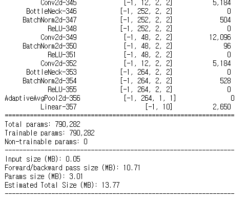

 모델 용량이 얼마 안되네요. 입력 이미지 사이즈가 작기 때문입니다. 마지막 conv layer에서 출력하는 피쳐맵 크기가 2x2밖에 안됩니다. 정확도를 높이기 위해서 입력 이미지 크기를 키워주는 것도 좋은 방법입니다.

 

3. 학습하기

 학습에 필요한 함수를 정의합니다.

# define loss function, optimizer, lr_scheduler
loss_func = nn.CrossEntropyLoss(reduction='sum')
opt = optim.Adam(model.parameters(), lr=0.01)

from torch.optim.lr_scheduler import ReduceLROnPlateau
lr_scheduler = ReduceLROnPlateau(opt, mode='min', factor=0.1, patience=8)


# get current lr
def get_lr(opt):
    for param_group in opt.param_groups:
        return param_group['lr']


# calculate the metric per mini-batch
def metric_batch(output, target):
    pred = output.argmax(1, keepdim=True)
    corrects = pred.eq(target.view_as(pred)).sum().item()
    return corrects


# calculate the loss per mini-batch
def loss_batch(loss_func, output, target, opt=None):
    loss_b = loss_func(output, target)
    metric_b = metric_batch(output, target)

    if opt is not None:
        opt.zero_grad()
        loss_b.backward()
        opt.step()
    
    return loss_b.item(), metric_b


# calculate the loss per epochs
def loss_epoch(model, loss_func, dataset_dl, sanity_check=False, opt=None):
    running_loss = 0.0
    running_metric = 0.0
    len_data = len(dataset_dl.dataset)

    for xb, yb in dataset_dl:
        xb = xb.to(device)
        yb = yb.to(device)
        output = model(xb)

        loss_b, metric_b = loss_batch(loss_func, output, yb, opt)

        running_loss += loss_b
        
        if metric_b is not None:
            running_metric += metric_b

        if sanity_check is True:
            break

    loss = running_loss / len_data
    metric = running_metric / len_data
    return loss, metric


# function to start training
def train_val(model, params):
    num_epochs=params['num_epochs']
    loss_func=params['loss_func']
    opt=params['optimizer']
    train_dl=params['train_dl']
    val_dl=params['val_dl']
    sanity_check=params['sanity_check']
    lr_scheduler=params['lr_scheduler']
    path2weights=params['path2weights']

    loss_history = {'train': [], 'val': []}
    metric_history = {'train': [], 'val': []}

    best_loss = float('inf')
    best_model_wts = copy.deepcopy(model.state_dict())
    start_time = time.time()

    for epoch in range(num_epochs):
        current_lr = get_lr(opt)
        print('Epoch {}/{}, current lr= {}'.format(epoch, num_epochs-1, current_lr))

        model.train()
        train_loss, train_metric = loss_epoch(model, loss_func, train_dl, sanity_check, opt)
        loss_history['train'].append(train_loss)
        metric_history['train'].append(train_metric)

        model.eval()
        with torch.no_grad():
            val_loss, val_metric = loss_epoch(model, loss_func, val_dl, sanity_check)
        loss_history['val'].append(val_loss)
        metric_history['val'].append(val_metric)

        if val_loss < best_loss:
            best_loss = val_loss
            best_model_wts = copy.deepcopy(model.state_dict())
            torch.save(model.state_dict(), path2weights)
            print('Copied best model weights!')

        lr_scheduler.step(val_loss)
        if current_lr != get_lr(opt):
            print('Loading best model weights!')
            model.load_state_dict(best_model_wts)

        print('train loss: %.6f, val loss: %.6f, accuracy: %.2f, time: %.4f min' %(train_loss, val_loss, 100*val_metric, (time.time()-start_time)/60))
        print('-'*10)

    model.load_state_dict(best_model_wts)
    return model, loss_history, metric_history

 val_loss가 낮을 때, 모델 가중치 파일을 자동으로 저장하도록 했습니다. 그리고 learning scheduler에 의해 학습률이 변화하면 val_loss가 낮을 때의 모델 가중치 파일을 불러오도록 했습니다.

 

 학습 파라미터를 설정합니다.

# define the training parameters
params_train = {
    'num_epochs':30,
    'optimizer':opt,
    'loss_func':loss_func,
    'train_dl':train_dl,
    'val_dl':val_dl,
    'sanity_check':False,
    'lr_scheduler':lr_scheduler,
    'path2weights':'./models/weights.pt',
}

# check the directory to save weights.pt
def createFolder(directory):
    try:
        if not os.path.exists(directory):
            os.makedirs(directory)
    except OSerror:
        print('Error')
createFolder('./models')

 

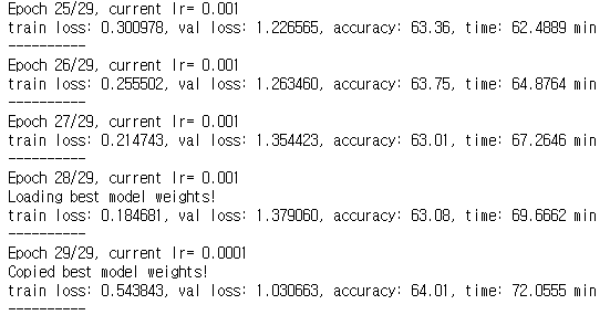
 학습을 진행하겠습니다. 30epoch로 설정했습니다.

model, loss_hist, metric_hist = train_val(model, params_train)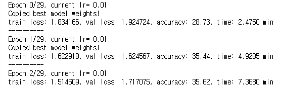

 

 loss와 accuracy progress를 확인하겠습니다.

# Train-Validation progress
num_epochs = params_train['num_epochs']

# plot loss progress
plt.title('Train-Val Loss')
plt.plot(range(1, num_epochs+1), loss_hist['train'], label='train')
plt.plot(range(1, num_epochs+1), loss_hist['val'], label='val')
plt.ylabel('Loss')
plt.xlabel('Training Epochs')
plt.legend()
plt.show()

# plot accuracy progress
plt.title('Train-Val Accuracy')
plt.plot(range(1, num_epochs+1), metric_hist['train'], label='train')
plt.plot(range(1, num_epochs+1), metric_hist['val'], label='val')
plt.ylabel('Accuracy')
plt.xlabel('Training Epochs')
plt.legend()
plt.show()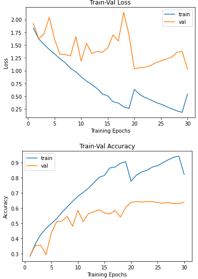

 감사합니다.