[논문 구현] PyTorch로 EfficientNet(2019) 구현하고 학습하기

 이번에 구현해볼 모델은 EfficientNet(2019) 입니다.

 

 EfficientNet은 강화학습으로 최적의 모델을 찾는 MnasNet의 구조를 사용합니다. MnasNet 구조에서 compound scaling을 적용하여 성능을 끌어올린 것이 EfficientNet입니다. compound scaling은 width, deepth, resolution 3가지 요소의 관계를 수식으로 정의해서 주어진 연산량에 맞게 효율적으로 width, deepth ,resolution를 조절하는 방법입니다. 자세한 논문 리뷰는 아래 포스팅에서 확인하실 수 있습니다.

[논문 읽기] EfficientNet(2019) 리뷰, Rethinking Model Scaling for Convolutional Neural Networks

 

 전체 코드는 여기에서 확인하실 수 있습니다.

 

1. 데이터셋 불러오기

 데이터셋은 torchvision 패키지에서 제공하는 STL10 dataset을 이용하겠습니다. STL10 dataset은 10개의 label을 갖으며 train dataset 5000개, test dataset 8000개로 구성됩니다.

 

 데이터셋을 불러오기 전에 Google Colab에 mount를 하고, 필요한 라이브러리를 import 하겠습니다.

from google.colab import drive
drive.mount('efficientnet')

# import package

# model
import torch
import torch.nn as nn
import torch.nn.functional as F
from torchsummary import summary
from torch import optim

# dataset and transformation
from torchvision import datasets
import torchvision.transforms as transforms
from torch.utils.data import DataLoader
from torchvision import models
import os

# display images
from torchvision import utils
import matplotlib.pyplot as plt
%matplotlib inline

# utils
import numpy as np
from torchsummary import summary
import time
import copy

 

 데이터셋을 불러옵니다.

# specify path to data
path2data = '/content/efficientnet/MyDrive/data'

# if not exists the path, make the directory
if not os.path.exists(path2data):
    os.mkdir(path2data)

# load dataset
train_ds = datasets.STL10(path2data, split='train', download=True, transform=transforms.ToTensor())
val_ds = datasets.STL10(path2data, split='test', download=True, transform=transforms.ToTensor())

print(len(train_ds))
print(len(val_ds))

 

 transformation을 정의하고, dataset에 적용합니다.

# define transformation
transformation = transforms.Compose([
                    transforms.ToTensor(),
                    transforms.Resize(224)
])

# apply transformation to dataset
train_ds.transform = transformation
val_ds.transform = transformation

# make dataloade
train_dl = DataLoader(train_ds, batch_size=32, shuffle=True)
val_dl = DataLoader(val_ds, batch_size=32, shuffle=True)

 

 샘플 이미지를 확인합니다.

# check sample images
def show(img, y=None):
    npimg = img.numpy()
    npimg_tr = np.transpose(npimg, (1, 2, 0))
    plt.imshow(npimg_tr)

    if y is not None:
        plt.title('labels:' + str(y))

np.random.seed(10)
torch.manual_seed(0)

grid_size=4
rnd_ind = np.random.randint(0, len(train_ds), grid_size)

x_grid = [train_ds[i][0] for i in rnd_ind]
y_grid = [val_ds[i][1] for i in rnd_ind]

x_grid = utils.make_grid(x_grid, nrow=grid_size, padding=2)
plt.figure(figsize=(10,10))
show(x_grid, y_grid)

 

2. 모델 구축하기

코드출처:

[1] https://github.com/zsef123/EfficientNets-PyTorch/blob/master/models/effnet.py

[2] https://github.com/katsura-jp/efficientnet-pytorch/blob/master/model/efficientnet.py

 

 위 코드를 바탕으로 좀 더 가독성이 있도록 수정을 했습니다.

 

 모델을 구축하기 전에 Swish 활성화 함수를 정의합니다.

# Swish activation function
class Swish(nn.Module):
    def __init__(self):
        super().__init__()
        self.sigmoid = nn.Sigmoid()

    def forward(self, x):
        return x * self.sigmoid(x)

# check
if __name__ == '__main__':
    x = torch.randn(3, 3, 224, 224)
    model = Swish()
    output = model(x)
    print('output size:', output.size())

 

 모델을 다 구축하고, check를 하면 오류가 발생했을 때 어디가 문제인지 파악하기 어려우므로 중간중간 확인을 했습니다.

 

 efficeintnet은 SE Block을 사용합니다. 따라서 SE Block도 정의하겠습니다.

# SE Block
class SEBlock(nn.Module):
    def __init__(self, in_channels, r=4):
        super().__init__()

        self.squeeze = nn.AdaptiveAvgPool2d((1,1))
        self.excitation = nn.Sequential(
            nn.Linear(in_channels, in_channels * r),
            Swish(),
            nn.Linear(in_channels * r, in_channels),
            nn.Sigmoid()
        )

    def forward(self, x):
        x = self.squeeze(x)
        x = x.view(x.size(0), -1)
        x = self.excitation(x)
        x = x.view(x.size(0), x.size(1), 1, 1)
        return x

# check
if __name__ == '__main__':
    x = torch.randn(3, 56, 17, 17)
    model = SEBlock(x.size(1))
    output = model(x)
    print('output size:', output.size())

 

 EfficientNet의 전체 구조는 다음과 같습니다. MBConv 클래스와 SepConv 클래스를 정의해야 합니다.

 

 EfficientNet에서 사용하는 MBConv입니다. 학습 시에 stochastic depth를 사용하므로 이 기능도 추가해야 합니다.

class MBConv(nn.Module):
    expand = 6
    def __init__(self, in_channels, out_channels, kernel_size, stride=1, se_scale=4, p=0.5):
        super().__init__()
        # first MBConv is not using stochastic depth
        self.p = torch.tensor(p).float() if (in_channels == out_channels) else torch.tensor(1).float()

        self.residual = nn.Sequential(
            nn.Conv2d(in_channels, in_channels * MBConv.expand, 1, stride=stride, padding=0, bias=False),
            nn.BatchNorm2d(in_channels * MBConv.expand, momentum=0.99, eps=1e-3),
            Swish(),
            nn.Conv2d(in_channels * MBConv.expand, in_channels * MBConv.expand, kernel_size=kernel_size,
                      stride=1, padding=kernel_size//2, bias=False, groups=in_channels*MBConv.expand),
            nn.BatchNorm2d(in_channels * MBConv.expand, momentum=0.99, eps=1e-3),
            Swish()
        )

        self.se = SEBlock(in_channels * MBConv.expand, se_scale)

        self.project = nn.Sequential(
            nn.Conv2d(in_channels*MBConv.expand, out_channels, kernel_size=1, stride=1, padding=0, bias=False),
            nn.BatchNorm2d(out_channels, momentum=0.99, eps=1e-3)
        )

        self.shortcut = (stride == 1) and (in_channels == out_channels)

    def forward(self, x):
        # stochastic depth
        if self.training:
            if not torch.bernoulli(self.p):
                return x

        x_shortcut = x
        x_residual = self.residual(x)
        x_se = self.se(x_residual)

        x = x_se * x_residual
        x = self.project(x)

        if self.shortcut:
            x= x_shortcut + x

        return x

# check
if __name__ == '__main__':
    x = torch.randn(3, 16, 24, 24)
    model = MBConv(x.size(1), x.size(1), 3, stride=1, p=1)
    model.train()
    output = model(x)
    x = (output == x)
    print('output size:', output.size(), 'Stochastic depth:', x[1,0,0,0])

 

 SepConv 입니다. MBConv와의 차이점은 expand=1인 것과 2개의 layer로 구성되어 있습니다. MBConv는 3개의 layer로 구정되어 있고, expand=6 입니다.

class SepConv(nn.Module):
    expand = 1
    def __init__(self, in_channels, out_channels, kernel_size, stride=1, se_scale=4, p=0.5):
        super().__init__()
        # first SepConv is not using stochastic depth
        self.p = torch.tensor(p).float() if (in_channels == out_channels) else torch.tensor(1).float()

        self.residual = nn.Sequential(
            nn.Conv2d(in_channels * SepConv.expand, in_channels * SepConv.expand, kernel_size=kernel_size,
                      stride=1, padding=kernel_size//2, bias=False, groups=in_channels*SepConv.expand),
            nn.BatchNorm2d(in_channels * SepConv.expand, momentum=0.99, eps=1e-3),
            Swish()
        )

        self.se = SEBlock(in_channels * SepConv.expand, se_scale)

        self.project = nn.Sequential(
            nn.Conv2d(in_channels*SepConv.expand, out_channels, kernel_size=1, stride=1, padding=0, bias=False),
            nn.BatchNorm2d(out_channels, momentum=0.99, eps=1e-3)
        )

        self.shortcut = (stride == 1) and (in_channels == out_channels)

    def forward(self, x):
        # stochastic depth
        if self.training:
            if not torch.bernoulli(self.p):
                return x

        x_shortcut = x
        x_residual = self.residual(x)
        x_se = self.se(x_residual)

        x = x_se * x_residual
        x = self.project(x)

        if self.shortcut:
            x= x_shortcut + x

        return x

# check
if __name__ == '__main__':
    x = torch.randn(3, 16, 24, 24)
    model = SepConv(x.size(1), x.size(1), 3, stride=1, p=1)
    model.train()
    output = model(x)
    # stochastic depth check
    x = (output == x)
    print('output size:', output.size(), 'Stochastic depth:', x[1,0,0,0])

 

 필요한 class를 다 정의했으므로 EfficeintNet을 정의합니다. 

class EfficientNet(nn.Module):
    def __init__(self, num_classes=10, width_coef=1., depth_coef=1., scale=1., dropout=0.2, se_scale=4, stochastic_depth=False, p=0.5):
        super().__init__()
        channels = [32, 16, 24, 40, 80, 112, 192, 320, 1280]
        repeats = [1, 2, 2, 3, 3, 4, 1]
        strides = [1, 2, 2, 2, 1, 2, 1]
        kernel_size = [3, 3, 5, 3, 5, 5, 3]
        depth = depth_coef
        width = width_coef

        channels = [int(x*width) for x in channels]
        repeats = [int(x*depth) for x in repeats]

        # stochastic depth
        if stochastic_depth:
            self.p = p
            self.step = (1 - 0.5) / (sum(repeats) - 1)
        else:
            self.p = 1
            self.step = 0


        # efficient net
        self.upsample = nn.Upsample(scale_factor=scale, mode='bilinear', align_corners=False)

        self.stage1 = nn.Sequential(
            nn.Conv2d(3, channels[0],3, stride=2, padding=1, bias=False),
            nn.BatchNorm2d(channels[0], momentum=0.99, eps=1e-3)
        )

        self.stage2 = self._make_Block(SepConv, repeats[0], channels[0], channels[1], kernel_size[0], strides[0], se_scale)

        self.stage3 = self._make_Block(MBConv, repeats[1], channels[1], channels[2], kernel_size[1], strides[1], se_scale)

        self.stage4 = self._make_Block(MBConv, repeats[2], channels[2], channels[3], kernel_size[2], strides[2], se_scale)

        self.stage5 = self._make_Block(MBConv, repeats[3], channels[3], channels[4], kernel_size[3], strides[3], se_scale)

        self.stage6 = self._make_Block(MBConv, repeats[4], channels[4], channels[5], kernel_size[4], strides[4], se_scale)

        self.stage7 = self._make_Block(MBConv, repeats[5], channels[5], channels[6], kernel_size[5], strides[5], se_scale)

        self.stage8 = self._make_Block(MBConv, repeats[6], channels[6], channels[7], kernel_size[6], strides[6], se_scale)

        self.stage9 = nn.Sequential(
            nn.Conv2d(channels[7], channels[8], 1, stride=1, bias=False),
            nn.BatchNorm2d(channels[8], momentum=0.99, eps=1e-3),
            Swish()
        ) 

        self.avgpool = nn.AdaptiveAvgPool2d((1,1))
        self.dropout = nn.Dropout(p=dropout)
        self.linear = nn.Linear(channels[8], num_classes)

    def forward(self, x):
        x = self.upsample(x)
        x = self.stage1(x)
        x = self.stage2(x)
        x = self.stage3(x)
        x = self.stage4(x)
        x = self.stage5(x)
        x = self.stage6(x)
        x = self.stage7(x)
        x = self.stage8(x)
        x = self.stage9(x)
        x = self.avgpool(x)
        x = x.view(x.size(0), -1)
        x = self.dropout(x)
        x = self.linear(x)
        return x


    def _make_Block(self, block, repeats, in_channels, out_channels, kernel_size, stride, se_scale):
        strides = [stride] + [1] * (repeats - 1)
        layers = []
        for stride in strides:
            layers.append(block(in_channels, out_channels, kernel_size, stride, se_scale, self.p))
            in_channels = out_channels
            self.p -= self.step

        return nn.Sequential(*layers)


def efficientnet_b0(num_classes=10):
    return EfficientNet(num_classes=num_classes, width_coef=1.0, depth_coef=1.0, scale=1.0,dropout=0.2, se_scale=4)

def efficientnet_b1(num_classes=10):
    return EfficientNet(num_classes=num_classes, width_coef=1.0, depth_coef=1.1, scale=240/224, dropout=0.2, se_scale=4)

def efficientnet_b2(num_classes=10):
    return EfficientNet(num_classes=num_classes, width_coef=1.1, depth_coef=1.2, scale=260/224., dropout=0.3, se_scale=4)

def efficientnet_b3(num_classes=10):
    return EfficientNet(num_classes=num_classes, width_coef=1.2, depth_coef=1.4, scale=300/224, dropout=0.3, se_scale=4)

def efficientnet_b4(num_classes=10):
    return EfficientNet(num_classes=num_classes, width_coef=1.4, depth_coef=1.8, scale=380/224, dropout=0.4, se_scale=4)

def efficientnet_b5(num_classes=10):
    return EfficientNet(num_classes=num_classes, width_coef=1.6, depth_coef=2.2, scale=456/224, dropout=0.4, se_scale=4)

def efficientnet_b6(num_classes=10):
    return EfficientNet(num_classes=num_classes, width_coef=1.8, depth_coef=2.6, scale=528/224, dropout=0.5, se_scale=4)

def efficientnet_b7(num_classes=10):
    return EfficientNet(num_classes=num_classes, width_coef=2.0, depth_coef=3.1, scale=600/224, dropout=0.5, se_scale=4)


# check
if __name__ == '__main__':
    device = torch.device('cuda' if torch.cuda.is_available() else 'cpu')
    x = torch.randn(3, 3, 224, 224).to(device)
    model = efficientnet_b0().to(device)
    output = model(x)
    print('output size:', output.size())

 

 model summry를 출력합니다.

# print model summary
model = efficientnet_b0().to(device)
summary(model, (3,224,224), device=device.type)

 

3. 학습하기

 학습에 필요한 함수를 정의하고, 학습을 하겠습니다.

# define loss function, optimizer, lr_scheduler
loss_func = nn.CrossEntropyLoss(reduction='sum')
opt = optim.Adam(model.parameters(), lr=0.01)

from torch.optim.lr_scheduler import ReduceLROnPlateau
lr_scheduler = ReduceLROnPlateau(opt, mode='min', factor=0.1, patience=10)


# get current lr
def get_lr(opt):
    for param_group in opt.param_groups:
        return param_group['lr']


# calculate the metric per mini-batch
def metric_batch(output, target):
    pred = output.argmax(1, keepdim=True)
    corrects = pred.eq(target.view_as(pred)).sum().item()
    return corrects


# calculate the loss per mini-batch
def loss_batch(loss_func, output, target, opt=None):
    loss_b = loss_func(output, target)
    metric_b = metric_batch(output, target)

    if opt is not None:
        opt.zero_grad()
        loss_b.backward()
        opt.step()
    
    return loss_b.item(), metric_b


# calculate the loss per epochs
def loss_epoch(model, loss_func, dataset_dl, sanity_check=False, opt=None):
    running_loss = 0.0
    running_metric = 0.0
    len_data = len(dataset_dl.dataset)

    for xb, yb in dataset_dl:
        xb = xb.to(device)
        yb = yb.to(device)
        output = model(xb)

        loss_b, metric_b = loss_batch(loss_func, output, yb, opt)

        running_loss += loss_b
        
        if metric_b is not None:
            running_metric += metric_b

        if sanity_check is True:
            break

    loss = running_loss / len_data
    metric = running_metric / len_data
    return loss, metric


# function to start training
def train_val(model, params):
    num_epochs=params['num_epochs']
    loss_func=params['loss_func']
    opt=params['optimizer']
    train_dl=params['train_dl']
    val_dl=params['val_dl']
    sanity_check=params['sanity_check']
    lr_scheduler=params['lr_scheduler']
    path2weights=params['path2weights']

    loss_history = {'train': [], 'val': []}
    metric_history = {'train': [], 'val': []}

    best_loss = float('inf')
    best_model_wts = copy.deepcopy(model.state_dict())
    start_time = time.time()

    for epoch in range(num_epochs):
        current_lr = get_lr(opt)
        print('Epoch {}/{}, current lr= {}'.format(epoch, num_epochs-1, current_lr))

        model.train()
        train_loss, train_metric = loss_epoch(model, loss_func, train_dl, sanity_check, opt)
        loss_history['train'].append(train_loss)
        metric_history['train'].append(train_metric)

        model.eval()
        with torch.no_grad():
            val_loss, val_metric = loss_epoch(model, loss_func, val_dl, sanity_check)
        loss_history['val'].append(val_loss)
        metric_history['val'].append(val_metric)

        if val_loss < best_loss:
            best_loss = val_loss
            best_model_wts = copy.deepcopy(model.state_dict())
            torch.save(model.state_dict(), path2weights)
            print('Copied best model weights!')

        lr_scheduler.step(val_loss)
        if current_lr != get_lr(opt):
            print('Loading best model weights!')
            model.load_state_dict(best_model_wts)

        print('train loss: %.6f, val loss: %.6f, accuracy: %.2f, time: %.4f min' %(train_loss, val_loss, 100*val_metric, (time.time()-start_time)/60))
        print('-'*10)

    model.load_state_dict(best_model_wts)
    return model, loss_history, metric_history

 

 학습 파라미터를 설정합니다.

# define the training parameters
params_train = {
    'num_epochs':100,
    'optimizer':opt,
    'loss_func':loss_func,
    'train_dl':train_dl,
    'val_dl':val_dl,
    'sanity_check':False,
    'lr_scheduler':lr_scheduler,
    'path2weights':'./models/weights.pt',
}

# check the directory to save weights.pt
def createFolder(directory):
    try:
        if not os.path.exists(directory):
            os.makedirs(directory)
    except OSerror:
        print('Error')
createFolder('./models')

 

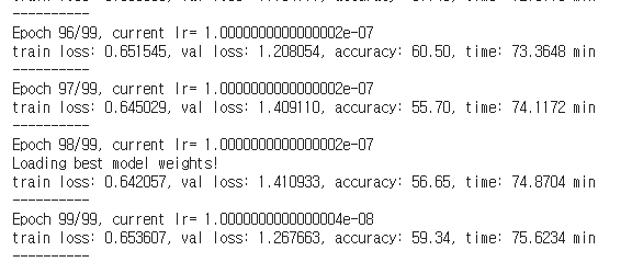
 100epoch 학습하겠습니다.

model, loss_hist, metric_hist = train_val(model, params_train)

 

 loss-accuracy progress를 출력합니다.

num_epochs = params_train['num_epochs']

# Plot train-val loss
plt.title('Train-Val Loss')
plt.plot(range(1, num_epochs+1), loss_hist['train'], label='train')
plt.plot(range(1, num_epochs+1), loss_hist['val'], label='val')
plt.ylabel('Loss')
plt.xlabel('Training Epochs')
plt.legend()
plt.show()

# plot train-val accuracy
plt.title('Train-Val Accuracy')
plt.plot(range(1, num_epochs+1), metric_hist['train'], label='train')
plt.plot(range(1, num_epochs+1), metric_hist['val'], label='val')
plt.ylabel('Accuracy')
plt.xlabel('Training Epochs')
plt.legend()
plt.show()

 

 

 파이토치로 efficientnet을 구현하고 학습해보았습니다. 감사합니다.