이 포스팅은 공부 목적으로 아래 게시물을 번역한 글입니다.
How to implement a YOLO (v3) object detector from scratch in PyTorch: Part 3
Part 3 of the tutorial series on how to implement a YOLO v3 object detector from scratch in PyTorch.
blog.paperspace.com
yolo v3을 파이토치로 바닥부터 구현하는 튜토리얼의 part 5 입니다. 지난 part에서 신경망의 출력값을 detection predictions로 변환하는 함수를 구현했습니다. 이제 남은 것은 입 출력 pipelines를 생성하는 것입니다.
전체 코드는 여기에서 확인하실 수 있습니다.
이 튜토리얼은 5가지로 나뉘어져 있습니다.
1. Part 1 : YOLO가 어떻게 작동하는지 이해하기
4. Part 4 : 비-최대 억제(Non-maximum suppression)와 객체 점수 임계값
5. Part 5 : (현재) 입력값과 출력값
이번 part에서 입 출력 pipeline을 구축할 것입니다. 이는 이미지를 읽고, prediction을 생성하고, 이미지에 bounding boxes를 그리기 위해 prediction을 사용하고, 그것들을 저장합니다. 또한 어떻게 detector이 카메라 또는 비디오에서 실시간으로 작동하는지에 대해 다룰것 입니다. 신경망의 다양한 하이퍼파라미터를 실험하는 command line도 소개할 것입니다. 이제 시작하겠습니다.
detector file에 detector.py를 생성합니다. 그리고 다음과 같이 import 합니다.
from __future__ import division
import time
import torch
import torch.nn as nn
from torch.autograd import Variable
import numpy as np
import cv2
from util import *
import argparse
import os
import os.path as osp
from darknet import Darknet
import pickle as pkl
import pandas as pd
import random
Command Line 인자 생성하기
detector.py 는 detector를 실행시키는 파일이기 때문에, 전달할 수 있는 좋은 command line 인자를 갖고 있어야 합니다. 이를 위해 ArgParse 모듈을 사용합니다.
def arg_parse():
    """
    detect module에 대한 인자 분석하기

    """

    parser = argparse.ArgumentParser(description='YOLO v3 Detection Module')

    parser.add_argument("--images", dest = 'images', help =
                        "Image / Directory containing images to perform detection upon",
                        default = "imgs", type = str)
    parser.add_argument("--det", dest = 'det', help =
                        "Image / Directory to store detections to",
                        default = "det", type = str)
    parser.add_argument("--bs", dest = "bs", help = "Batch size", default = 1)
    parser.add_argument("--confidence", dest = "confidence", help = "Object Confidence to filter predictions", default = 0.5)
    parser.add_argument("--nms_thresh", dest = "nms_thresh", help = "NMS Threshhold", default = 0.4)
    parser.add_argument("--cfg", dest = 'cfgfile', help =
                        "Config file",
                        default = "cfg/yolov3.cfg", type = str)
    parser.add_argument("--weights", dest = 'weightsfile', help =
                        "weightsfile",
                        default = "yolov3.weights", type = str)
    parser.add_argument("--reso", dest = 'reso', help =
                        "Input resolution of the network. Increase to increase accuracy. Decrease to increase speed",
                        default = "416", type = str)

    return parser.parse_args()

args = arg_parse()
images = args.images
batch_size = int(args.bs)
confidence = float(args.confidence)
nms_thesh = float(args.nms_thresh)
start = 0
CUDA = torch.cuda.is_available()
이중에서, 중요한 flag는 images(입력 이미지 및 이미지의 directory를 명시하기 위해 사용됩니다), det(detectors를 저장하는 Directory), reso(입력 이미지 해상도, 속도-정확도의 균형을 위해 사용됩니다.), cfg(configuration file), weightfile 입니다.
신경망 불러오기
coco.names 파일을 여기서 다운 받습니다. 파일은 COCO dataset에 있는 객체들의 이름을 포함합니다. detector directory에 data 폴더를 생성합니다.
그리고나서, 프로그램에 class 파일을 불러옵니다.
num_classes = 80    #For COCO
classes = load_classes("data/coco.names")
load_classes는 util.py에서 정의되어, 모든 class의 index와 이름 string을 매핑하는 dictionary를 반환하는 함수입니다.
def load_classes(namesfile):
    fp = open(namesfile, "r")
    names = fp.read().split("\n")[:-1]
    return names
신경망을 초기화하고 weights를 불러옵니다.
# 신경망 설정하기
print("Loading network.....")
model = Darknet(args.cfgfile)
model.load_weights(args.weightsfile)
print("Network successfully loaded")

model.net_info["height"] = args.reso
inp_dim = int(model.net_info["height"])
assert inp_dim % 32 == 0
assert inp_dim > 32

# GPU가 사용가능하면, GPU에서 모델 구동하기
if CUDA:
    model.cuda()

# model을 evaluation mode로 설정하기
model.eval()
입력 이미지 읽기
입력 이미지를 읽습니다. 이미지의 경로는 imlist 에 저장됩니다.
read_dir = time.time()
#Detection phase
try:
    imlist = [osp.join(osp.realpath('.'), images, img) for img in os.listdir(images)]
except NotADirectoryError:
    imlist = []
    imlist.append(osp.join(osp.realpath('.'), images))
except FileNotFoundError:
    print ("No file or directory with the name {}".format(images))
    exit()
read_dir은 시간을 측정하기 위해 사용되는 checkpoint입니다. (이것을 여러번 사용할 것입니다.)
만약 def flag로 정의된 detections를 저장하기 위한 directory가 없다면 생성합니다.
if not os.path.exists(args.det):
    os.makedirs(args.det)
이미지를 불러오기 위해 OpenCV를 사용할 것입니다.
load_batch = time.time()
loaded_ims = [cv2.imread(x) for x in imlist]
load_batch 는 다른 checkpoint 입니다.
OpenCV는 이미지를 BGR 컬러 채널 순서를 가진 numpy array로 불러옵니다. PyTorch의 이미지 입력 형식은 RGB 채널 순서를 지닌 (Batches x Channels x Height x Width) 입니다. 그러므로 numpy array를 PyTorch의 입력 형식으로 변환하기 위해 util.py에 있는 prep_image 함수를 작성합니다.
이 함수를 작성하기 전에, 이미지를 resize하고, aspect ratio를 일정하게 유지하고, 남은 영역을 (128, 128, 128) 색상으로 패딩하는 letterbox_image 함수를 작성해야 합니다.
def letterbox_image(img, inp_dim):
    ''' padding을 사용하여 aspect ratio가 변화하지 않고 이미지를 resize 합니다.'''
    img_w, img_h = img.shape[1], img.shape[0]
    w, h = inp_dim
    new_w = int(img_w * min(w/img_w, h/img_h))
    new_h = int(img_h * min(w/img_w, h/img_h))
    resized_image = cv2.resize(img, (new_w,new_h), interpolation = cv2.INTER_CUBIC)

    canvas = np.full((inp_dim[1], inp_dim[0], 3), 128)

    canvas[(h-new_h)//2:(h-new_h)//2 + new_h,(w-new_w)//2:(w-new_w)//2 + new_w,  :] = resized_image

    return canvas
이제, OpenCV 이미지를 취하고 신경망의 입력으로 전환하는 함수를 작성하겠습니다.
def prep_image(img, inp_dim):
    """
    신경망에 입력하기 위한 이미지 준비
    변수를 반환합니다.
    """

    img = cv2.resize(img, (inp_dim, inp_dim))
    img = img[:,:,::-1].transpose((2,0,1)).copy()
    img = torch.from_numpy(img).float().div(255.0).unsqueeze(0)
    return img
변환된 이미지 이외에도, 기존 이미지의 list와 기존 이미지의 차원을 담고있는 list im_dim_list 를 유지합니다.
# 이미지를 위한 PyTorch Variables
im_batches = list(map(prep_image, loaded_ims, [inp_dim for x in range(len(imlist))]))

# 기존 이미지의 차원을 담고 있는 List
im_dim_list = [(x.shape[1], x.shape[0]) for x in loaded_ims]
im_dim_list = torch.FloatTensor(im_dim_list).repeat(1,2)

if CUDA:
    im_dim_list = im_dim_list.cuda()
배치 생성하기
leftover = 0
if (len(im_dim_list) % batch_size):
   leftover = 1

if batch_size != 1:
   num_batches = len(imlist) // batch_size + leftover
   im_batches = [torch.cat((im_batches[i*batch_size : min((i +  1)*batch_size,
                       len(im_batches))]))  for i in range(num_batches)]
Detection Loop
이제 배치를 반복하고 prediction을 생성하고 detection을 수행한 모든 이미지의 prediction tensors를 연결합니다. tensor의 shape는 Dx8이고, write_results 함수의 출력입니다.)
각 배치에서, 입력을 받고 write_result 함수의 출력이 생성되기 까지 걸리는 시간을 측정합니다. write_prediction에 의해 반환된 출력에서, 속성중 하나는 배치에서 이미지의 index입니다. 특정 속성을 모든 이미지의 주소를 담고 있는 list인 imlist에 있는 이미지의 index를 나타내는 방식으로 변환합니다.
그 이후에, 각 이미지에서 검출된 object뿐만 아니라 각 detection에 걸리는 시간을 출력합니다.
만약 배치당 write_results 함수의 추력값이 int(0)이면, detection이 존재하지 않다는 것을 의미하고 남은 loop를 건너뛰기 위해 continue를 사용합니다.
write = 0
start_det_loop = time.time()
for i, batch in enumerate(im_batches):
    # 이미지 불러오기
    start = time.time()
    if CUDA:
        batch = batch.cuda()

    prediction = model(Variable(batch, volatile = True), CUDA)

    prediction = write_results(prediction, confidence, num_classes, nms_conf = nms_thesh)

    end = time.time()

    if type(prediction) == int:

        for im_num, image in enumerate(imlist[i*batch_size: min((i +  1)*batch_size, len(imlist))]):
            im_id = i*batch_size + im_num
            print("{0:20s} predicted in {1:6.3f} seconds".format(image.split("/")[-1], (end - start)/batch_size))
            print("{0:20s} {1:s}".format("Objects Detected:", ""))
            print("----------------------------------------------------------")
        continue

    prediction[:,0] += i*batch_size    # 배치에있는 index 속성을 imlist에서 index 속성으로 변환합니다.

    if not write:                      # 출력값이 초기화되지 않은 경우
        output = prediction
        write = 1
    else:
        output = torch.cat((output,prediction))

    for im_num, image in enumerate(imlist[i*batch_size: min((i +  1)*batch_size, len(imlist))]):
        im_id = i*batch_size + im_num
        objs = [classes[int(x[-1])] for x in output if int(x[0]) == im_id]
        print("{0:20s} predicted in {1:6.3f} seconds".format(image.split("/")[-1], (end - start)/batch_size))
        print("{0:20s} {1:s}".format("Objects Detected:", " ".join(objs)))
        print("----------------------------------------------------------")

    if CUDA:
        torch.cuda.synchronize()
torch.cuda.synchronize line을 사용하면 CUDA kernel이 CPU와 동기화됩니다. 그렇지 않으면, CUDA kernel은 GPU가 대기중이 되자마자 CPU에 컨트롤을 되돌리고, GPU 작업이 끝나기 전에 CPU에 컨트롤을 되돌립니다. 이것은 아마 GPU 작업이 정확하게 끝나기 전에 end = time.time()이 출력됩니다.
이제, Tensor Output에 있는 모든 이미지의 detections를 갖게 됬습니다. 이미지에 bounding boxes를 그려보겠습니다.
이미지에 bounding boxes 그리기
detection이 생성되었는지 안되었는지 확인하기 위해 try-catch block을 사용합니다.
try:
    output
except NameError:
    print ("No detections were made")
    exit()
bounding boxes를 그리기 전에, 출력 tensor에 포함된 predictions는 기존 이미지의 크기가 아닌 신경망의 입력 사이즈를 따릅니다. 그래서, bounding boxes를 그리기 전에, 각 bounding box의 꼭지점 인자를 이미지의 원래 차원으로 변환합니다.
또한 predictions는 기존 이미지가 아닌 패딩된 이미지로 얻은 prediction입니다. 단지, 그것들을 입력 이미지의 차원으로 re-scaling 하는 것은 도움이 되지 않습니다. 첫 번째로 boxes 좌표를 원래 이미지를 포함하는 패딩된 이미지에 대한 영역의 경계를 고려하여 변환합니다.
# 패딩된 이미지에 대한 영역의 경계를 고려하여 바운딩박스의 좌표 변환
im_dim_list = torch.index_select(im_dim_list, 0, output[:,0].long())

scaling_factor = torch.min(inp_dim/im_dim_list,1)[0].view(-1,1)


output[:,[1,3]] -= (inp_dim - scaling_factor*im_dim_list[:,0].view(-1,1))/2
output[:,[2,4]] -= (inp_dim - scaling_factor*im_dim_list[:,1].view(-1,1))/2
이제, 좌표는 패딩된 영역에 대한 이미지의 차원을 따릅니다. 하지만, letterbox_image 함수에서, scaling 인자(차원을 aspect ratio를 유지하기 위해 공통된 인자로 나눴습니다.)에 의해 이미지의 차원을 resize 했습니다. 이제 기존 이미지에 대한 bounding box의 좌표를 얻기 위해 이 rescaling을 되돌립니다.
# 기존 이미지에 대한 바운딩 박스의 좌표를 얻기 위해 rescaling 되돌리기
output[:,1:5] /= scaling_factor
이제 bounding boxes를 잘라냅니다.
# 바운딩박스 잘라내기
for i in range(output.shape[0]):
    output[i, [1,3]] = torch.clamp(output[i, [1,3]], 0.0, im_dim_list[i,0])
    output[i, [2,4]] = torch.clamp(output[i, [2,4]], 0.0, im_dim_list[i,1])
많약 이미지에 많은 bounding boxes가 있으면, 하나의 색으로 모두 그리는 것은 좋은 생각이 아닙니다. 이 파일을 detector 폴더에 다운로드 하세요. 이것은 임의로 선택할 수 있는 여러 색이 포함된 pickled file 입니다.
class_load = time.time()
colors = pkl.load(open("pallete", "rb"))
이제 boxes를 그리는 함수를 작성하겠습니다.
draw = time.time()

def write(x, results, color):
    c1 = tuple(x[1:3].int())
    c2 = tuple(x[3:5].int())
    img = results[int(x[0])]
    cls = int(x[-1])
    label = "{0}".format(classes[cls])
    cv2.rectangle(img, c1, c2,color, 1)
    t_size = cv2.getTextSize(label, cv2.FONT_HERSHEY_PLAIN, 1 , 1)[0]
    c2 = c1[0] + t_size[0] + 3, c1[1] + t_size[1] + 4
    cv2.rectangle(img, c1, c2,color, -1)
    cv2.putText(img, label, (c1[0], c1[1] + t_size[1] + 4), cv2.FONT_HERSHEY_PLAIN, 1, [225,255,255], 1);
    return img
colors로부터 임의로 선택된 색상으로 사각형을 그리는 함수입니다. 또한 bounding box의 왼쪽 상단에 class가 적혀있는 사각형도 작성합니다. cv2.rectangle 함수의 -1 인자는 색칠된 사각형을 생성합니다.
colors list에 접근하기 위해서 write 함수를 정의합니다.
list(map(lambda x: write(x, loaded_ims), output))
위의 짧은 코드는 loaded_ims 안에 있는 이미지들을 차례차례 수정합니다.
각 이미지들은 이미지 이름의 앞에 'det__'를 사전에 고정하여 저장합니다. detection 이미지들을 저장할 주소 목록을 생성합니다.
det_names = pd.Series(imlist).apply(lambda x: "{}/det_{}".format(args.det,x.split("/")[-1]))
마지막으로 detections를 지닌 이미지들을 det_names 주소로 저장합니다.
list(map(cv2.imwrite, det_names, loaded_ims))
end = time.time()
시간 요약본 출력하기
detector의 마지막에 코드가 얼마나 오랫동안 실행됬는지를 나타내는 요약본을 출력합니다. 이것은 detector의 속도에 하이퍼파라미터가 얼마나 영향을 미쳤는지 비교할 때 유용합니다. batch size, objectness confidence, NMS threshold와 같은 하이퍼파라미터들은 명령줄에서 detection.py가 실행되는 동안에 설정될 수 있습니다.
print("SUMMARY")
print("----------------------------------------------------------")
print("{:25s}: {}".format("Task", "Time Taken (in seconds)"))
print()
print("{:25s}: {:2.3f}".format("Reading addresses", load_batch - read_dir))
print("{:25s}: {:2.3f}".format("Loading batch", start_det_loop - load_batch))
print("{:25s}: {:2.3f}".format("Detection (" + str(len(imlist)) +  " images)", output_recast - start_det_loop))
print("{:25s}: {:2.3f}".format("Output Processing", class_load - output_recast))
print("{:25s}: {:2.3f}".format("Drawing Boxes", end - draw))
print("{:25s}: {:2.3f}".format("Average time_per_img", (end - load_batch)/len(imlist)))
print("----------------------------------------------------------")


torch.cuda.empty_cache()
Object Detector 시험하기
terminal에서 실행해보겠습니다.
python detect.py --images dog-cycle-car.png --det det
출력값을 생성합니다.
Loading network.....
Network successfully loaded
dog-cycle-car.png    predicted in  2.456 seconds
Objects Detected:    bicycle truck dog
----------------------------------------------------------
SUMMARY
----------------------------------------------------------
Task                     : Time Taken (in seconds)

Reading addresses        : 0.002
Loading batch            : 0.120
Detection (1 images)     : 2.457
Output Processing        : 0.002
Drawing Boxes            : 0.076
Average time_per_img     : 2.657
----------------------------------------------------------
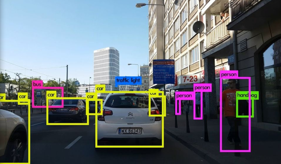
det 디렉토리에 저장된 det_dog-cycle-car.png 이미지입니다.

'Python > PyTorch 공부' 카테고리의 다른 글
| [PyTorch] 암 이미지로 커스텀 데이터셋 만들기(creating custom dataset for cancer images) (0) | 2021.02.22 |
|---|---|
| [PyTorch] CNN 신경망 구축하고 MNIST 데이터셋으로 학습하기 (1) | 2021.02.14 |
| [Object Detection] YOLO(v3)를 PyTorch로 바닥부터 구현하기 - Part 4 (0) | 2021.01.29 |
| [Object Detection] YOLO(v3)를 PyTorch로 바닥부터 구현하기 - Part 3 (6) | 2021.01.25 |
| [Object Detection] YOLO(v3)를 PyTorch로 바닥부터 구현하기 - Part 2 (8) | 2021.01.11 |