반응형
코드 출처
[1] https://github.com/JWarmenhoven/ISLR-python
[2] https://github.com/emredjan/ISL-python
선형 회귀(Linear Regression)
필요한 라이브러리 import
# 필요한 라이브러리 import
import pandas as pd
import numpy as np
import matplotlib.pyplot as plt
from mpl_toolkits.mplot3d import axes3d
import seaborn as sns

from sklearn.preprocessing import scale
import sklearn.linear_model as skl_lm
from sklearn.metrics import mean_squared_error, r2_score
import statsmodels.api as sm
import statsmodels.formula.api as smf

%matplotlib inline
plt.style.use('seaborn-white')
데이터셋 불러오기
https://github.com/emredjan/ISL-python 에 업로드 되어 있는 데이터 셋을 불러와서 사용하겠습니다.
# 깃허브를 클론합니다.
!git clone https://github.com/emredjan/ISL-python
# Advertising.csv 데이터셋을 불러옵니다.
advertising = pd.read_csv('/content/ISL-python/datasets/Advertising.csv', usecols=[1,2,3,4])
advertising.info() # 정보 출력
# credit.csv 데이터셋을 불러옵니다.
credit = pd.read_csv('/content/ISL-python/datasets/Credit.csv', usecols=list(range(1,12)))
credit['Student2'] = credit.Student.map({'No':0, 'Yes':1}) # 범주형 자료를 수치형 자료로 변경
credit.head(3) # 위에서 세번째 행까지 출력, Student2 열이 수치형으로 나타납니다.
# Auto.csv 데이터셋을 불러옵니다.
auto = pd.read_csv('/content/ISL-python/datasets/Auto.csv', na_values='?').dropna()
auto.info()
3.1 단순 선형 회귀(Simple Linear Regression)
- 단순 선형 회귀는 설명 변수(predictor)이 하나인 경우를 의미합니다.
- RSS(residual sum of squared)를 최소화하는 방향으로 설명 변수의 계수(coefficient)를 추정합니다.
# 데이터를 점으로 나타내면서 선형성도 함께 나타냅니다.
sns.regplot(advertising.TV, advertising.Sales, order=1, ci=None, scatter_kws={'color':'r', 's':9})
plt.xlim(-10,310)
plt.ylim(ymin=0);
RSS
- 반응 변수: sales
- 설명 변수: TV
- 단순 선형 회귀를 수행합니다.
- 절편과 TV 계수에 따른 RSS 값을 시각화 합니다.
# sales에 대한 TV의 선형 회귀 계수를 추정합니다.
regress = skl_lm.LinearRegression()

X = scale(advertising.TV, with_mean=True, with_std=False).reshape(-1,1)
y = advertising.Sales

regress.fit(X,y)
print('절편: ',regress.intercept_) # 절편
print('TV 계수: ', regress.coef_)
# 절편과 계수 시각화
B0 = np.linspace(regress.intercept_-2, regress.intercept_+2, 50) # 절편의 구간 설정
B1 = np.linspace(regress.coef_-0.02, regress.coef_+0.02, 50) # TV 계수의 구간 설정
xx, yy = np.meshgrid(B0, B1, indexing='xy') # 그리드 생성
Z = np.zeros((B0.size, B1.size)) # 계수에 따른 RSS 결과값을 담을 배열 생성

# 계수를 기반으로 Z값(RSS) 계산
for (i, j),v in np.ndenumerate(Z):
    Z[i,j] = ((y-(xx[i,j]+X.ravel()*yy[i,j]))**2).sum()/float(1000)

# RSS 최소화
min_RSS = r'$\beta_0$, $\beta_1$ for minimized RSS'
# RSS = (y - b0 - b1*X)**2
min_rss = np.sum((regress.intercept_+regress.coef_*X - y.values.reshape(-1,1))**2)/1000
print('RSS 최소값: ',min_rss)
# 시각화
fig = plt.figure(figsize=(15,6))
fig.suptitle('RSS - 회귀 계수', fontsize=20)

ax1 = fig.add_subplot(121)
ax2 = fig.add_subplot(122, projection='3d')

# 왼쪽 plot
CS = ax1.contour(xx, yy, Z, cmap=plt.cm.Set1, levels=[2.15, 2.2, 2.3, 2.5, 3])
ax1.scatter(regress.intercept_, regress.coef_[0], c='r', label=min_RSS)
ax1.clabel(CS, inline=True, fontsize=10, fmt='%1.1f')

# 오른쪽 plot
ax2.plot_surface(xx, yy, Z, rstride=3, cstride=3, alpha=0.3)
ax2.contour(xx, yy, Z, zdir='z', offset=Z.min(), cmap=plt.cm.Set1,
            alpha=0.4, levels=[2.15, 2.2, 2.3, 2.5, 3])
ax2.scatter3D(regress.intercept_, regress.coef_[0], min_rss, c='r', label=min_RSS)
ax2.set_zlabel('RSS')
ax2.set_zlim(Z.min(),Z.max())
ax2.set_ylim(0.02,0.07)

# plot 설정
for ax in fig.axes:
    ax.set_xlabel(r'$\beta_0$', fontsize=17)
    ax.set_ylabel(r'$\beta_1$', fontsize=17)
    ax.set_yticks([0.03,0.04,0.05,0.06])
    ax.legend()
통계값 출력
- 반응 변수: Sales
- 설명 변수: TV
est = smf.ols('Sales ~ TV', advertising).fit()
est.summary().tables[1]
# RSS = sales - 절편 - 회귀계수 * TV
RSS = ((advertising.Sales - (est.params[0] + est.params[1]*advertising.TV))**2).sum()/1000
print('최소 RSS:', RSS)
계수 추정
- 반응 변수: Sales
- 설명 변수: TV
regress = skl_lm.LinearRegression()

X = advertising.TV.values.reshape(-1,1)
y = advertising.Sales

regress.fit(X,y)
print('절편:',regress.intercept_)
print('TV 계수:', regress.coef_)
R2 test
Sales_pred = regress.predict(X)
r2 = r2_score(y, Sales_pred)
print('R2 test:', r2)
3.2 다중 선형 회귀(Multiple Linear Regression)
Sales에 대한 TV, Radio, Newspaper 세 가지 변수 각각 단순 선형 회귀로 계수 추정
# TV
est = smf.ols('Sales ~ TV', advertising).fit()
est.summary().tables[1]
# Radio
est = smf.ols('Sales ~ Radio', advertising).fit()
est.summary().tables[1]
# Newspaper
est = smf.ols('Sales ~ Newspaper', advertising).fit()
est.summary().tables[1]
세 가지 변수 다중 선형 회귀
- F 통계량을 도출하여, Sales가 세 가지 변수중 적어도 한가지 이상 변수와 연관되어 있는지 확인합니다.
est = smf.ols('Sales ~ TV + Radio + Newspaper', advertising).fit()
est.summary()
상관행렬(correlation matrix)
advertising.corr()
Radio, TV 두 변수 다중 선형 회귀
# 계수 추정
regress = skl_lm.LinearRegression()

X = advertising[['Radio', 'TV']]
y = advertising.Sales

regress.fit(X,y)
print('Radio와 TV의 계수:', regress.coef_)
print('절편:',regress.intercept_)
# 통계값 출력
advertising[['Radio', 'TV']].describe()
다중 선형 회귀 시각화
- 반응 변수: sales
- 설명 변수: TV, Radio
# 좌표 grid 생성
Radio = np.arange(0,50)
TV = np.arange(0,300)

B1, B2 = np.meshgrid(Radio, TV, indexing='xy')
Z = np.zeros((TV.size, Radio.size))

for (i,j),v in np.ndenumerate(Z):
        Z[i,j] =(regress.intercept_ + B1[i,j]*regress.coef_[0] + B2[i,j]*regress.coef_[1])

# plot 생성
fig = plt.figure(figsize=(10,6))
fig.suptitle('Regression: Sales ~ Radio + TV Advertising', fontsize=20)

ax = axes3d.Axes3D(fig)

ax.plot_surface(B1, B2, Z, rstride=10, cstride=5, alpha=0.4)
ax.scatter3D(advertising.Radio, advertising.TV, advertising.Sales, c='r')

ax.set_xlabel('Radio')
ax.set_xlim(0,50)
ax.set_ylabel('TV')
ax.set_ylim(ymin=0)
ax.set_zlabel('Sales');
3.3 여러 경우에서 회귀 모델
질적 자료
sns.pairplot(credit[['Balance','Age','Cards','Education','Income','Limit','Rating']]);
더미 변수를 생성하여 질적 자료 수치화
library에서 자동으로 더미 변수를 생성하는 것 같습니다.
# 반응 변수: 신용카드대금
# 설명 변수: 성별
est = smf.ols('Balance ~ Gender', credit).fit()
est.summary().tables[1]
# 반응 변수: 신용카드대금
# 설명 변수: 인종
est = smf.ols('Balance ~ Ethnicity', credit).fit()
est.summary().tables[1]
TV와 Radio의 상호 작용 효과
- 상호 작용 term을 추가하여 회귀 분석
est = smf.ols('Sales ~ TV + Radio + TV*Radio', advertising).fit()
est.summary().tables[1]
양적 자료와 질적 자료 사이의 상호 작용
# 반응 변수: Balance
# 설명 변수: 학생, 수입

# 상호작용 없이
est1 = smf.ols('Balance ~ Income + Student2', credit).fit()
regress1 = est1.params
# 상호작용
est2 = smf.ols('Balance ~ Income + Income*Student2', credit).fit()
regress2 = est2.params

print('Regression 1 - without interaction term')
print(regress1)
print('\nRegression 2 - with interaction term')
print(regress2)
# 시각화

income = np.linspace(0,150) # x-axis

# 상호 작용 없이 Balance 값 (y-axis)
student1 = np.linspace(regress1['Intercept']+regress1['Student2'],
                       regress1['Intercept']+regress1['Student2']+150*regress1['Income'])
non_student1 =  np.linspace(regress1['Intercept'], regress1['Intercept']+150*regress1['Income'])

# 상호 작용을 추가한 Balance 값 (y-axis)
student2 = np.linspace(regress2['Intercept']+regress2['Student2'],
                       regress2['Intercept']+regress2['Student2']+
                       150*(regress2['Income']+regress2['Income:Student2']))
non_student2 =  np.linspace(regress2['Intercept'], regress2['Intercept']+150*regress2['Income'])

# plot 생성하기
fig, (ax1,ax2) = plt.subplots(1,2, figsize=(12,5))
ax1.plot(income, student1, 'r', income, non_student1, 'k')
ax2.plot(income, student2, 'r', income, non_student2, 'k')

for ax in fig.axes:
    ax.legend(['student', 'non-student'], loc=2)
    ax.set_xlabel('Income')
    ax.set_ylabel('Balance')
    ax.set_ylim(ymax=1550)
비선형 관계
# 데이터 산점도
plt.scatter(auto.horsepower, auto.mpg, facecolors='None', label='mpg', edgecolors='k', alpha=.5)

# 단순 선형 회귀
sns.regplot(auto.horsepower, auto.mpg, ci=None, label='Linear', scatter=False, color='orange')

# 2차 다항 선형 회귀
sns.regplot(auto.horsepower, auto.mpg, ci=None, label='Degree 2', order=2, scatter=False, color='lightblue')

# 5차 다항 선형 회귀
sns.regplot(auto.horsepower, auto.mpg, ci=None, label='Degree 5', order=5, scatter=False, color='g')

plt.legend()
plt.ylim(5,55)
plt.xlim(40,240);
2차 다항 선형 회귀
# X ** 2 변수 생성
auto['horsepower2'] = auto.horsepower**2
auto.head(3)
# 2차 다항 선형 회귀
est = smf.ols('mpg ~ horsepower + horsepower2', auto).fit()
est.summary().tables[1]
잔차 그래프
- 잔차 그래프를 시각화하여 설명 변수와 반응 변수 사이의 비-선형 관계를 식별할 수 있습니다.
regress = skl_lm.LinearRegression()

# 선형 적합
X = auto.horsepower.values.reshape(-1,1) # 설명 변수 1개
y = auto.mpg
regress.fit(X, y)

auto['pred1'] = regress.predict(X)
auto['resid1'] = auto.mpg - auto.pred1

# 2차 형식 적합
X2 = auto[['horsepower', 'horsepower2']] # 2차 계수항 추가
regress.fit(X2, y)

auto['pred2'] = regress.predict(X2)
auto['resid2'] = auto.mpg - auto.pred2
# 잔차 그래프 시각화
fig, (ax1,ax2) = plt.subplots(1,2, figsize=(12,5))
# 왼쪽 plot, 선형 fit에 대한 잔차 그래프
sns.regplot(auto.pred1, auto.resid1, lowess=True,
ax=ax1, line_kws={'color':'r', 'lw':1},
scatter_kws={'facecolors':'None', 'edgecolors':'k', 'alpha':0.5})
ax1.hlines(0,xmin=ax1.xaxis.get_data_interval()[0],
xmax=ax1.xaxis.get_data_interval()[1], linestyles='dotted')
ax1.set_title('Residual Plot for Linear Fit')
# 오른쪽 plot, 2차 fit에 대한 잔차 그래프
sns.regplot(auto.pred2, auto.resid2, lowess=True,
line_kws={'color':'r', 'lw':1}, ax=ax2,
scatter_kws={'facecolors':'None', 'edgecolors':'k', 'alpha':0.5})
ax2.hlines(0,xmin=ax2.xaxis.get_data_interval()[0],
xmax=ax2.xaxis.get_data_interval()[1], linestyles='dotted')
ax2.set_title('Residual Plot for Quadratic Fit')
for ax in fig.axes:
ax.set_xlabel('Fitted values')
ax.set_ylabel('Residuals')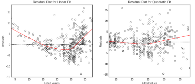
공선성(Colinearity)
fig, (ax1,ax2) = plt.subplots(1,2, figsize=(12,5))

# 왼쪽 plot
ax1.scatter(credit.Limit, credit.Age, facecolor='None', edgecolor='r')
ax1.set_ylabel('Age')

# 오른쪽 plot
ax2.scatter(credit.Limit, credit.Rating, facecolor='None', edgecolor='r')
ax2.set_ylabel('Rating')

for ax in fig.axes:
    ax.set_xlabel('Limit')
    ax.set_xticks([2000,4000,6000,8000,12000])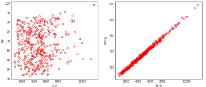
공선성을 지니는 두 설명 변수에 대한 RSS 시각화
- 공선성이 존재하는 경우에 추정된 계수값은 높은 불확실성을 갖습니다.
- 즉, 매우 넓은 표준 오차를 초래합니다.
y = credit.Balance # 반응 변수: Balance

# 설명 변수: Age, Limint
X = credit[['Age', 'Limit']]
regress1 = skl_lm.LinearRegression()
regress1.fit(scale(X.astype('float'), with_std=False), y)
print('Age/Limit\n',regress1.intercept_)
print(regress1.coef_)

# 설명 변수: Rating, Limit (강한 공선성 존재)
X2 = credit[['Rating', 'Limit']]
regress2 = skl_lm.LinearRegression()
regress2.fit(scale(X2.astype('float'), with_std=False), y)
print('\nRating/Limit\n',regress2.intercept_)
print(regress2.coef_)
# 그리드 좌표 생성하기
B_Age = np.linspace(regress1.coef_[0]-3, regress1.coef_[0]+3, 100)
B_Limit = np.linspace(regress1.coef_[1]-0.02, regress1.coef_[1]+0.02, 100)

B_Rating = np.linspace(regress2.coef_[0]-3, regress2.coef_[0]+3, 100)
B_Limit2 = np.linspace(regress2.coef_[1]-0.2, regress2.coef_[1]+0.2, 100)

X1, Y1 = np.meshgrid(B_Limit, B_Age, indexing='xy')
X2, Y2 = np.meshgrid(B_Limit2, B_Rating, indexing='xy')
Z1 = np.zeros((B_Age.size,B_Limit.size))
Z2 = np.zeros((B_Rating.size,B_Limit2.size))

Limit_scaled = scale(credit.Limit.astype('float'), with_std=False)
Age_scaled = scale(credit.Age.astype('float'), with_std=False)
Rating_scaled = scale(credit.Rating.astype('float'), with_std=False)

# 계수에 기반한 RSS
for (i,j),v in np.ndenumerate(Z1):
    Z1[i,j] =((y - (regress1.intercept_ + X1[i,j]*Limit_scaled +
                    Y1[i,j]*Age_scaled))**2).sum()/1000000

for (i,j),v in np.ndenumerate(Z2):
    Z2[i,j] =((y - (regress2.intercept_ + X2[i,j]*Limit_scaled +
                    Y2[i,j]*Rating_scaled))**2).sum()/1000000
fig = plt.figure(figsize=(12,5))
fig.suptitle('RSS - Regression coefficients', fontsize=20)
ax1 = fig.add_subplot(121)
ax2 = fig.add_subplot(122)
min_RSS = r'$\beta_0$, $\beta_1$ for minimized RSS'
# 왼쪽 plot: 공선성이 없는 두 설명 변수
CS = ax1.contour(X1, Y1, Z1, cmap=plt.cm.Set1, levels=[21.25, 21.5, 21.8])
ax1.scatter(regress1.coef_[1], regress1.coef_[0], c='r', label=min_RSS)
ax1.clabel(CS, inline=True, fontsize=10, fmt='%1.1f')
ax1.set_ylabel(r'$\beta_{Age}$', fontsize=17)
# 오른쪽 plot: 강한 공선성이 존재하는 두 설명 변수
CS = ax2.contour(X2, Y2, Z2, cmap=plt.cm.Set1, levels=[21.5, 21.8])
ax2.scatter(regress2.coef_[1], regress2.coef_[0], c='r', label=min_RSS)
ax2.clabel(CS, inline=True, fontsize=10, fmt='%1.1f')
ax2.set_ylabel(r'$\beta_{Rating}$', fontsize=17)
ax2.set_xticks([-0.1, 0, 0.1, 0.2])
for ax in fig.axes:
ax.set_xlabel(r'$\beta_{Limit}$', fontsize=17)
ax.legend()
VIF(Variance Inflation Factor) 계산
- VIF는 다중 공선성을 판별하기 위해 사용합니다.
est_Age = smf.ols('Age ~ Rating + Limit', credit).fit()
est_Rating = smf.ols('Rating ~ Age + Limit', credit).fit()
est_Limit = smf.ols('Limit ~ Age + Rating', credit).fit()

print('Age의 VIF: ', 1/(1-est_Age.rsquared))
print('Rating의 VIF', 1/(1-est_Rating.rsquared))
print('Limit의 VIF', 1/(1-est_Limit.rsquared))
참고자료 및 그림 출처
Gareth James의 An Introduction to Statistical Learning
반응형
'수학 > Statistical Learning' 카테고리의 다른 글
| [ISLR] 수축법(Shrinkage Methods), 능형 회귀(Ridge regression) (1) | 2021.05.31 |
|---|---|
| [ISLR] Cp, AIC, BIC, Adjusted R2, 검증 및 교차검증(Validation and Cross-Validation) (0) | 2021.05.30 |
| [ISLR] 부분집합 선택(Subset Selection), 최상의 부분 집합, 전진 단계적, 후진 단계적, 하이브리드 (0) | 2021.05.30 |
| [ISLR] 교차검증(Cross-validation), K-Fold, LOOCV (0) | 2021.05.09 |
| [ISLR] Classification - Logistic Regression, LDA, QDA, KNN (0) | 2021.05.08 |